Cross Entropy Demistified
Understanding the maths behind Cross Entropy Loss
Understanding “Entropy”, “Cross-Entropy Loss” and “KL Divergence”
Classification is one of the preliminary steps in most Machine Learning and Deep learning projects and Cross-Entropy Loss is the most commonly used loss function, but have you ever tried to explore what is cross-entropy or entropy exactly.
Ever imagined why cross-entropy works for classification?
This series of articles consisting of 2 parts is designed to explain in detail the intuition behind what is cross-entropy and why cross-entropy has been used as the most popular cost function for classification.
Before diving into cross-entropy loss and its application to classification, the concept of entropy and cross-entropy must be clear, so this article is dedicated to exploring what these 2 terms mean.
The content and images in this post are inspired by the amazing tutorial A Short Introduction to Entropy, Cross-Entropy and KL-Divergence by Aurélien Géron
Entropy
The concept of entropy and cross-entropy comes from Claude Shannon’s Information theory which he introduces through his classical paper “A Mathematical Theory of Communication”
According to Shannon, Entropy is the minimum no of useful bits required to transfer information from a sender to a receiver.
Let’s understand the two terms by looking into an example.
Suppose that we need to share the weather information of a place with another friend who stays in a different city, and the weather has a 50–50 chance of being sunny or rainy every day.

This information can be transmitted using just a single bit (0 or 1) and the uncertainty associated with this event is 2 as there are 2 possibilities, either weather is sunny or rainy.
If the probability of occurrence of an event is , then the uncertainty raised due to that event is given as
In our example, the probability of occurrence of both events is 0.5 so the uncertainty for each event is
Even if the information is transferred as a string “RAINY” having 5 characters each of 1 byte, the total information transferred is 40 bits but only 1 bit of useful information is transferred.
Given the uncertainty due to an event is , the minimum number of bits required to transfer the information about that event can be calculated as
Here, as uncertainty for weather being rainy or sunny is 2, the minimum no. of useful bits required to transfer information about being sunny or rainy is
Note : In the article, means logarithm with base and means natural logarithm with base
Now suppose that the event “Weather” had 8 possibilities, all equally likely with probability of occurrence of each.

So now as the no. of uncertainties is 8, the minimum no. of useful bits required to transfer information about each event can be calculated as
Let us consider a case which is similar to the 1st case that we saw with 2 possibilities, sunny or rainy, but now both are not equally likely. One occurs with a probability of and the other with a probability of .

Now the events are not occuring with equal probabilities, so the uncertainties for the events will be different. the uncertainty of the weather being rainy is and for the weather being sunny is
The minimum number of useful bits required the information is rainy is and for the weather being sunny is
This also be derived from the probability directly as, given the probability of a given event is , then the uncertainty associated with the occurrence of that event is and hence the minimum number of useful bits required to transfer information about it is,
2 bits are required to say whether the weather is rainy and 0.4 bits are required to say if the weather is sunny, so the average no. of useful bits required to transmit the information can be calculated as,
So on average, we would receive 0.81 bits of information and this is the minimum number of bits required to transfer the weather information, following the above-mentioned probability distribution.This is known as Entropy.
Entropy (expressed in ‘bits’) is a measure of how unpredictable the probability distribution is. So more the individual events vary, the more is its entropy.
Cross-Entropy
Cross entropy is the average message length that is used to transmit the message.

In this example, there are 8 variations all equally likely. So the entropy of this system is 3, but suppose that the probability distribution changes with probabilities something like this :

Though the probability distribution has changed, we still use 3 bits to transfer this information.
Now the entropy of this distribution will be,
which is the minimum number of useful bits transmitted, and entropy of the system.
So though we are sending 3 bits of information, the user gets 2.23 useful bits. This can be improved by changing the no. of bits used to address each kind of information. Suppose we use a following distribution :

The average no. of bits transmitted using the following bit pattern is,
which is close to the entropy. This is the Cross Entropy
But suppose the same bit pattern is used for a different probability distribution :

which is significantly grater than the entropy.
This happens because the bit code we are using is making some implicit estimation of the probability distribution of the weather as,
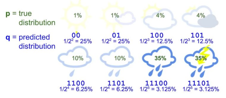
So we can express cross-entropy as a function of both the true distribution and predicted distribution as,
Here instead of taking the of the true probability, we are taking the of the predicted probability distribution .
Basically, when we know the probability of occurrence of the events, but we don’t know the bit distribution of the events, so a random distribution can be taken and given the probabilities and assumed bit distribution, cross-entropy of the events can be calculated and cross-checked with the original entropy to see if the assumed distribution gives the minimum uncertainty for the given probabilities or not. Hence it is termed as “Cross” entropy.
Usually Cross entropy is larger than the entropy of a distribution. When the predicted distribution is equal to true distribution, the cross-entropy is equal to entropy.
Kullback–Leibler Divergence
The amount by which the cross-entropy exceeds the entropy is called Relative Entropy or commonly known as Kullback-Leibler Divergence or KL Divergence.
So the key take away from this article is,
given a probability distribution, the minimum average no. of useful bits required to transfer the information about the distribution is its Entropy which can also be said as the minimum possible randomness that can be associated with a probability distribution.
In the last example, we took an assumed bit distribution for each event and found the cross-entropy of that distribution with the original probabilities of the events. This cross-entropy resulted to be higher than the original entropy. So we tried to change the assumed bit distribution so that we can reduce the cross-entropy and make it as close as possible to the entropy.
But wait for a second !!
Isn’t that exactly what we try to do in a classification?
We start with a randomly initialized model that outputs an assumed bit distribution for the different classes that we want to classify, and in the process of training, we try to achieve an optimal distribution that can get us close enough to the lowest possible Entropy for the probability distribution.
So does that mean cross-entropy can be used to quantify how bad is the model performing in assuming the distribution?
Can we use KL Divergence as a metric to measure how bad the model is performing?
In the subsequent article, we shall explore the answer to all these questions and understand the intuition behind why Cross-Entropy is an appropriate loss function for our requirement.
Got some doubts/suggestions?
Please feel free to share your suggestions, questions, queries, and doubts through comments below — I will be happy to talk/discuss them all.